Capital market assumptions – what do we put a premium on?
14 Aug 2020 - Estimated reading time: 2 mins
A widely held belief underpinning asset allocation decisions for long-term investors is that higher risk assets, on average, outperform lower risk assets. This (expected, not guaranteed) outperformance is known as a risk premium1.
In the context of DB pensions, risk premiums are consequential assumptions influencing the choice of investment strategy, and level of contributions. As a result, there are often discussions/disagreements/bunfights around what the ‘correct’ risk premiums should be for different asset classes.
This blog examines the assumption that there exists a ‘correct’ risk premium for different asset classes and explores the implications if this belief is shaky. For ease we’ll focus on the most famous example – the equity risk premium (“ERP”).
First, some modelling.
Let’s pretend that equity returns all come from an unseen, unchanging, ‘true’ distribution (we don’t actually know this but bear with us). How much return data do we need before we can infer, with some reasonable degree of confidence, what the true expected return on equity is?
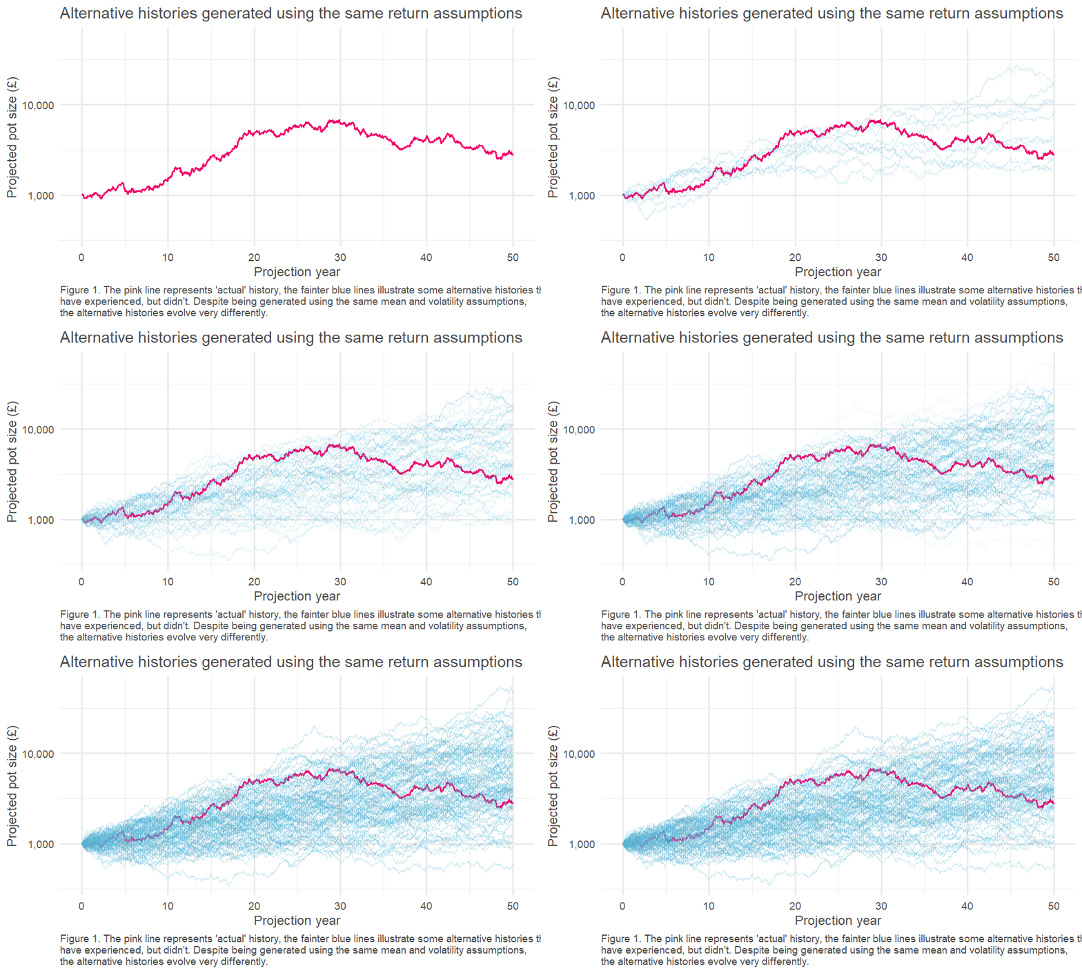
We can test this by running many simulations, with all returns generated randomly from our ‘true’ distribution2. This is an example of a well-known technique called Monte Carlo modelling3. One of the benefits of this approach is that we can explore many ‘simulated histories,’ which is helpful, given we only have one ‘actual history’ to guide us.
Click picture to enlarge
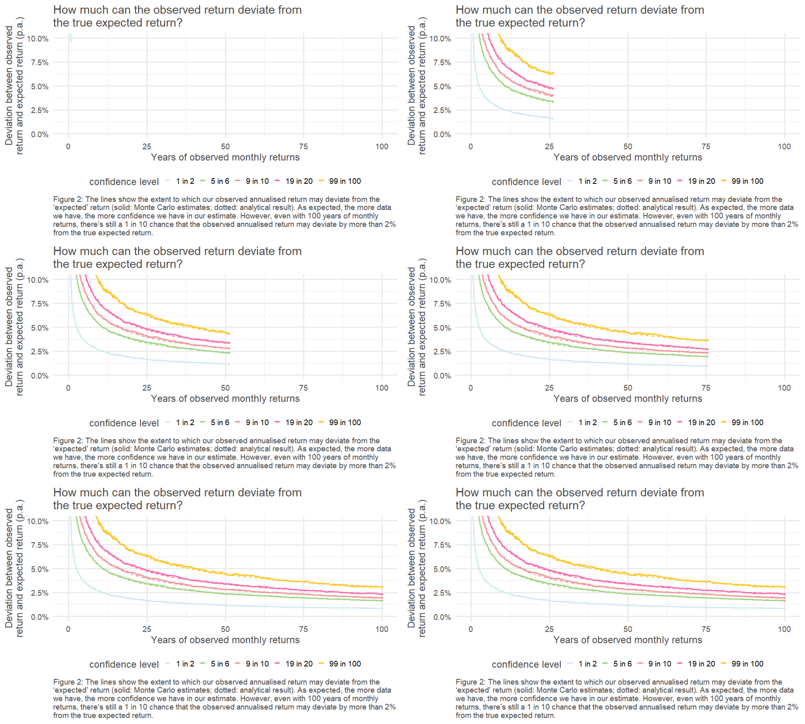
This, in turn, means we can look at the spread of outcomes driven by the randomness of the underlying return process. This is charted below – how quickly do our observed (annualised) returns converge on the underlying ‘true’ average return?4
Click picture to enlarge
The results are stark: even for equities, the asset class for which we’ve got the most historical data5, we can only pin down our error range to c. +/- 1% if we want to have the same confidence as a coin flip. The variability of the historically observed returns year on year clouds our estimate of the true expected return.
This shows that there’s a fair degree of uncertainty in pinning down an ERP. However, this ‘parameter uncertainty’ is often ignored in long-term financial modelling, where a two-step process is typically followed:
- Calibrate an economic scenario generator (choosing values for parameters like the ERP in the process); and
- Use scenarios from the economic scenario generator in order to explore the long run risk/return profile of alternative investment strategies.
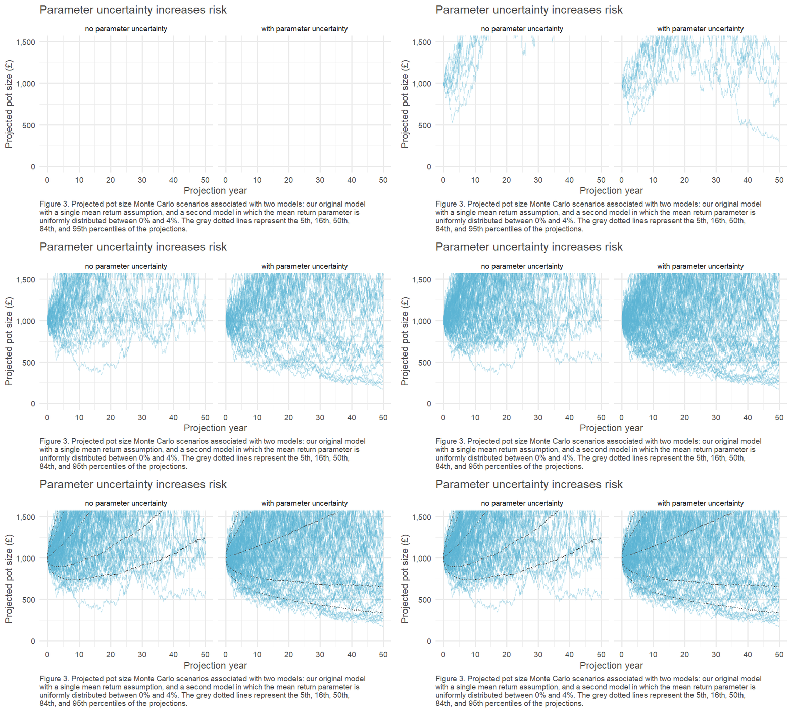
Does ignoring parameter uncertainty really matter? Well, what if we happen (by chance) to have been overly optimistic when calibrating the ERP? Below we compare the range of investment outcomes under our example where we the expected return is known and fixed, versus a situation where we allow this expected return to vary randomly at a level below this point estimate6.
Click picture to enlarge
When we ignore parameter uncertainty, the likelihood that equity will lose money over a multi-decade horizon is remote; however, when we allow for parameter uncertainty, this is clearly a much more tangible possibility.
We’re not suggesting that modelling is useless. A model is simply a tool that enables us to explore the consequences of our assumptions about the future in a controlled way. It is designed to help the user profit; it is not designed to be a prophet. Modelling risk is as much about communicating the risks which aren’t captured within the framework as it is about understanding those which are.
It ain’t what you know that gets you into trouble. It’s what you know for sure that just ain’t so.
Unknown -
1. The technical definition of a ‘risk premium’ is the expected outperformance above the risk-free rate (i.e. return above cash).
2. We’ve assumed that continuously compounded returns are normally distributed with a mean of 4% p.a., and a standard deviation of 12%. We’re not claiming this is a particularly good fit – in particular, it’s well known that equity returns exhibit heavier tails than this. However, if equity exhibits more unpredictability than assumed here (which we believe it does) this only strengthens the argument. Also, we’re being fairly loose in terms of moving between ‘returns’ and ‘risk premium.’ For the purposes of this simulation, we’ve ignored interest rates by assuming that the risk-free rate is fixed at 0% (which is potentially less implausible as a forward looking assumption than it might have been in the past!), which would imply the risk premium and the return are equivalent.
3. This type of analysis is used extensively in the institutional investment industry as a risk management and valuation tool. There are additional complexities around refining the distributions to more closely match observed data, and wrinkles around using alternative probability measures for different purposes, but it’s the same fundamental idea.
4. Helpfully, given the choice of underlying return process, the distribution of the sample mean is also known (it’s a normal distribution). This is illustrated by the dotted line.
5. Available, for example, in the form of the BarCap equity gilt study, which runs back to c. 1900.
6. In the first case, we set the expected return at 4%. In the latter, we allow it to vary uniformly between 0-4%. Bearing in mind that it would take 30 years of data to pin our estimate down to + / - 1.5% with a 1-in-2 confidence level, if anything it could be argued this remains a tight range.


0 comments on this post